User Interface Walkthrough
The graphical user interface (GUI) for MicroGridsPy offers a user-friendly platform for defining and inputting data, organized into specialized pages catering to different model aspects. It facilitates comprehensive data input and validation, ensuring accuracy through tooltips and validation mechanisms across various input fields such as basic parameters, RES time series, and technology configurations. With dynamic parameter management, the interface adapts to user selections, enabling or disabling options in real-time, streamlining the input process, and enhancing decision-making through effective visualization. Additionally, it provides efficient run functionalities, allowing users to track progress and visualize results seamlessly, thereby optimizing the modeling process for enhanced efficiency.
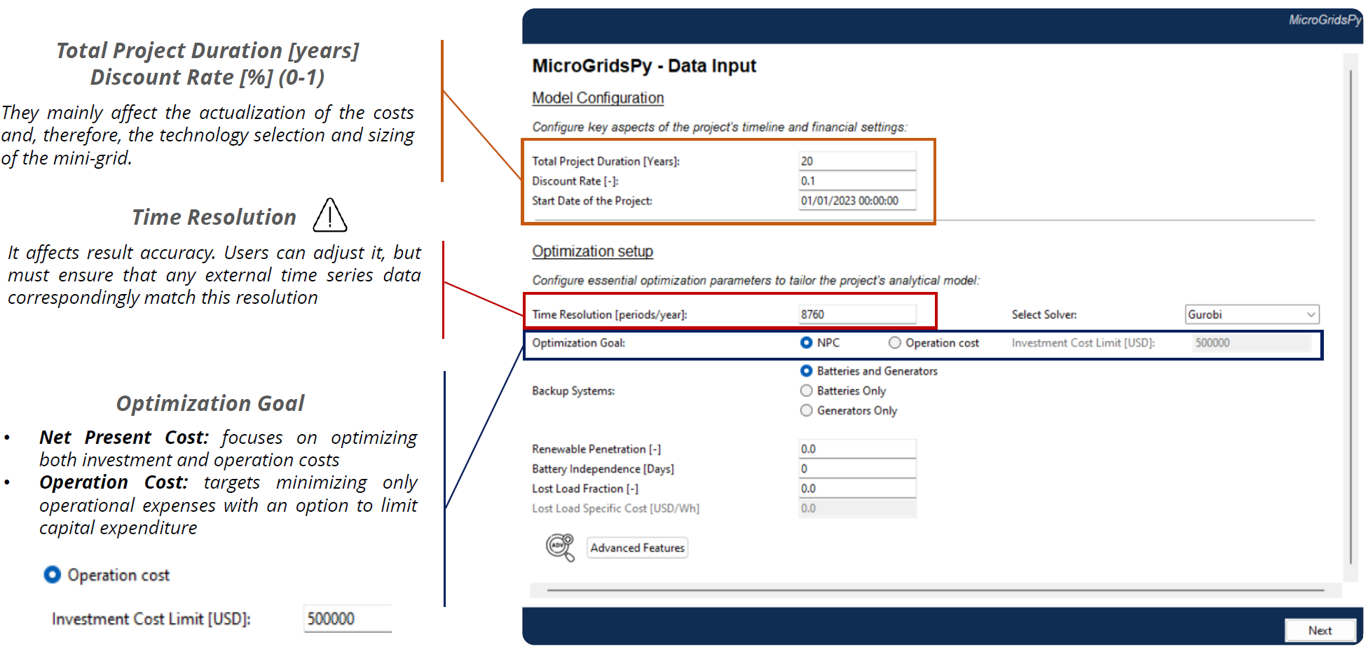
Model configuration
This first section of the GUI is designed to configure the key aspects of your project’s timeline and financial settings. Users can specify the total duration of the project in years and set the discount rate as a decimal to impact the actuarial considerations of the costs, which will influence the selection and sizing of the mini-grid technologies. In the Optimization Setup, users can tailor essential parameters to fit project’s analytical model. This includes setting the Time Resolution in periods per year and choosing the Optimization goal between net present cost and operation cost, with the former focusing on both investment and operation costs and the latter on operational expenses with an option to limit capital expenditure. The Time Resolution field can be adjusted to impact the accuracy of the results. It requires careful consideration, especially when integrating external time series data, to ensure matching resolution.
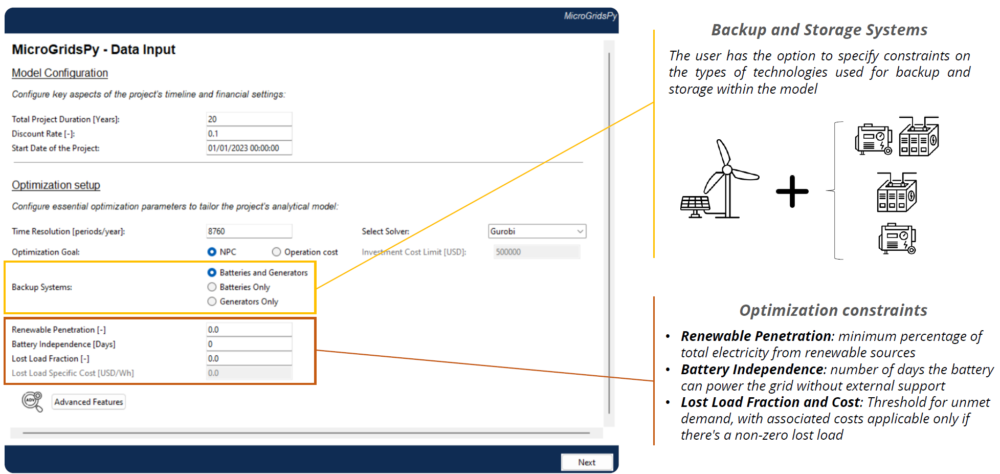
Users can set constraints on the types of technologies used for backup and storage within the model. This option enables the selection among batteries and generators, batteries only, or generators only. This choice determines the flexibility and resilience of the power supply in the face of variable renewable energy outputs and consumption patterns. The interface allows users to set important optimization constraints that affect the performance of the mini-grid:
Renewable Penetration: This parameter sets the minimum percentage of total electricity that must come from renewable sources, ensuring that the project meets sustainability goals.
Battery Independence: Indicates the number of days the battery storage system can power the grid without external support, which is crucial for reliability in off-grid or unstable grid scenarios.
Lost Load Fraction and Cost: Defines the threshold for unmet demand, along with associated costs that apply only if there is a non-zero lost load. This helps to quantify the impact of shortages and prioritize reliability in the system design.
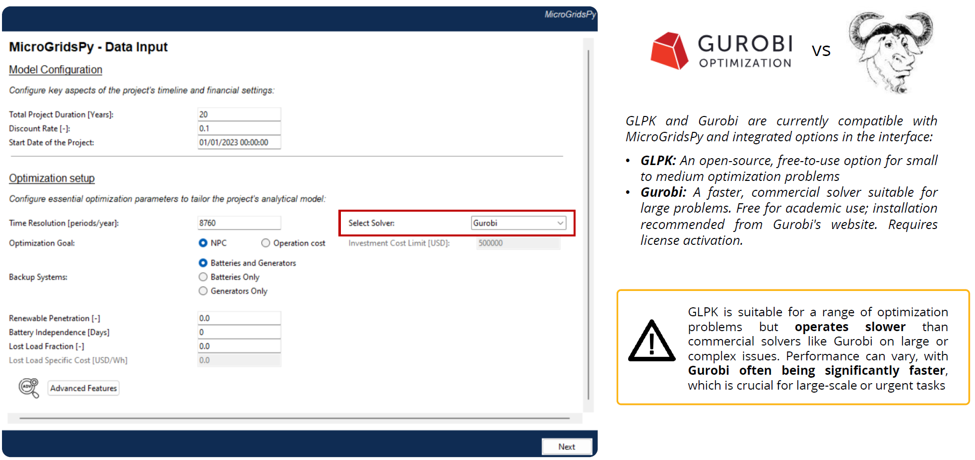
Two solvers are (currently) available and integrated in MicroGridsPy:
GLPK: The GNU Linear Programming Kit (GLPK) is an open-source solver that is suitable for solving small to medium-sized optimization problems. It is a cost-effective solution that can handle various linear optimization tasks.
Gurobi: For larger and more complex problems, Gurobi is the recommended solver. It is a commercial solver known for its high performance and speed, making it ideal for academic and professional use where large-scale optimization tasks are involved. Although it requires license activation, Gurobi is free for academic use, and installation instructions can be obtained from the official Gurobi website.
Important Note: While GLPK is an adequate choice for many scenarios, its performance may be slower compared to commercial solvers like Gurobi, especially when dealing with large-scale or complex optimization problems. Therefore, it is recommended to consider the size and complexity of your microgrid project when choosing the solver to ensure efficient computation times and optimization results.
Advanced features
By clicking the Advanced Features button, the section offers a suite of enhanced modeling options and configurations that extend beyond basic settings.
Advanced Modeling Options:
Capacity Expansion: This feature allows planning for additional capacity requirements as the project grows over time. If capacity Expansion is activated, users can also specify:
Step Duration [Years]: Users can determine the time increments for the model to evaluate capacity expansion.
Minimum Last Step Duration [Years]: This sets the mandatory duration for the last expansion step, ensuring stability in the project’s growth phase.
LP vs MILP Formulation: Linear Programming (LP) approaches provide a simplified, continuous representation of operations, ideal for scenarios where decisions do not need to be binary. Mixed-Integer Linear Programming (MILP), however, incorporates integer variables, allowing for a unit commitment approach that can handle on/off decisions and more complex relationships, crucial for discrete decision-making processes like those found in many energy systems. Delving into the MILP formulation of the model, additional and more advanced modeling equations could be integrated. Currently, if MILP is activated:
Generator Partial Load: Allows for the inclusion of generator partial load characteristics in the model, optimizing the operation of generators according to their load profiles.
Considering the investment strategy:
Greenfield vs. Brownfield: Users can select between a new site development (Greenfield) or an upgrade to existing infrastructure (Brownfield), affecting investment strategies and costs.
Grid Connection:
On-grid vs. Off-grid: This determines whether the microgrid will be connected to a larger grid or operate independently.
Grid Availability: Users can activate this setting if grid availability is variable and should be considered in the model.
Grid Connection Type: Offers a choice between purchase-only or the ability to both purchase and sell electricity, reflecting the microgrid’s interaction with the main grid.
For financial modeling:
WACC Calculation: Activating this computes the Weighted Average Cost of Capital, integrating the cost implications of both debt and equity financing into the project’s financial planning.
Expanding on cost calculations:
Fuel Specific Cost Calculation: This feature enables users to estimate the variable costs of fuel over time, considering both the initial cost and the rate of change.
When configuring the optimization process:
Multi-Objective Optimization: This advanced feature goes beyond single-objective cost minimization by also considering emissions. It provides a mechanism for building a Pareto Curve, which represents various trade-offs between cost and emissions. Users can select the number of Pareto points to analyze, allowing them to explore the spectrum of solutions from minimizing emissions to minimizing costs. The interface also enables users to choose and display a specific solution on this curve, facilitating informed decision-making based on environmental impact and economic factors.
Multi-Scenario Optimization: This allows for the evaluation of different operational scenarios within a single run, providing valuable insights into potential performance under varying conditions.

Resource Assessment
The Resource Assessment interface is designed to meticulously calculate the potential of renewable energy sources at the project’s location. The GUI also includes an automated function to endogenously calculate the RES time series. By activating the RES Time Series Calculation, the model will estimate the electricity output of renewable generation units using NASA POWER data, which necessitates an internet connection.
Input the latitude and longitude in DMS format to accurately define the geographical positioning of your project, which is fundamental for resource assessment.
Specify solar PV parameters, which include the nominal power of the solar panels, tilt angle, azimuth, and efficiency-related coefficients, to precisely model the solar generation potential.
Specify wind turbine parameters for wind energy estimation, select the turbine type and model from the provided list. Details like the turbine’s rated power and drivetrain efficiency are essential to accurately calculate wind energy generation potential.

If this automatic calculation is deactivated, users are responsible for supplying the RES Time Series Data as a CSV file. The CSV file, named RES_Time_Series.csv, should be placed within the Code/Model/Inputs directory. Data within the CSV file should represent the hourly electricity output for each renewable source unit over an entire year. Each column in the CSV file corresponds to a different renewable source, and the columns should be numbered sequentially to match the total number of renewable units considered. Rows represent consecutive hours throughout the year, starting from the first hour of January 1st to the last hour of December 31st. The values are expected to be in watts (W), reflecting the output power produced by each unit for every hour. Please ensure the CSV file is formatted correctly, as any discrepancies in the data structure can lead to inaccuracies in the model’s output or potential errors in the simulation.

Load Demand Assessment
The Load Demand Assessment interface allows users to forecast the electricity demand based on socioeconomic factors and service needs within the community. It caters to both endogenous estimation using built-in profiles and the inclusion of exogenous demand time series data. If Demand Time Series Calculation is activated, the model will estimate the electricity demand using predefined profiles (archetypes) that represent different user categories, such as households and public services. They are valid just for Sub-Sahara Africa. The demand drivers, like anticipated annual demand growth and seasonal cooling periods, can be adjusted. Choose from ‘No Cooling’ (NC), ‘All Year’ (AY), ‘Oct-Mar’ (OM), or ‘Apr-Sept’ (AS) to reflect the expected seasonal variations in energy usage. Users need to specify the number of households across various wealth tiers to reflect the socioeconomic diversity of the village, which affects the ownership and use of energy-intensive appliances and enter the number of educational and healthcare facilities in the village, with tiers representing the range from rural dispensaries to sub-county hospitals, as well as the typical load for a rural primary school.

For incorporating externally calculated or historical demand data, deactivate the Demand Profile Generation and supply the demand time series as a CSV file located in the Code/Inputs/Demand.csv. The CSV file must contain hourly electricity demand in watts for each year of the time horizon, structured with numbered columns corresponding to each year. Users must ensure the rows represent consecutive hours through the year, providing a detailed time series of demand.

Both endogenous and exogenous approaches to load demand estimation are critical for accurately modeling and planning the mini-grid’s capacity and operational strategy. Correct configuration and data input are essential to reflect the unique characteristics and requirements of the location being served.
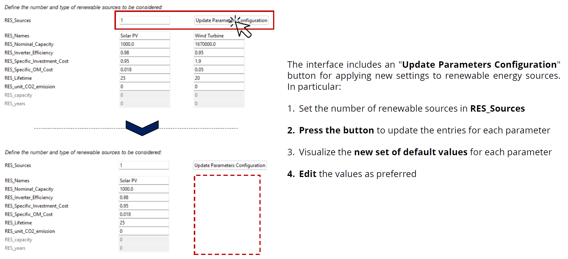
Renewables Characterization
The GUI’s Renewables Characterization interface provides a streamlined process for specifying the attributes of different renewable energy sources. Users can define a variety of parameters such as types, capacities, efficiencies, and costs which are essential for accurate simulation of renewable technologies. The interface is designed to be flexible, accommodating a range of renewable energy technologies and their respective attributes. The number and types of renewable sources are set under the RES_Sources field, which then enables the configuration of parameters for each selected technology. The interface page includes a Update Parameters Configuration button, which applies the new settings to the renewable energy sources. After setting the number of renewable sources and adjusting the necessary parameters, pressing this button will update the system with the latest configurations. In-depth control over the configuration allows for the activation of additional parameters based on the selected advanced features, providing the flexibility to adapt the model to specific project needs such as brownfield or greenfield investments.

Storage System Characterization
The Storage System Characterization interface facilitates the definition of battery bank parameters, playing a crucial role in the energy storage aspect of a minigrid design. Within this section: Users can input key parameters related to battery systems such as investment costs, operational costs, efficiencies, lifecycle, and CO2 emissions. The flexibility of the interface allows for the activation or deactivation of certain parameters based on the advanced features selected, like MILP modeling and brownfield investment considerations.

Backup System Characterization
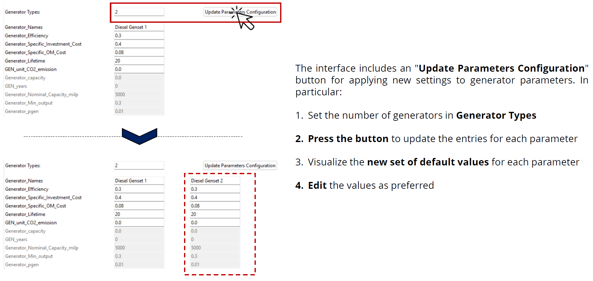
The Backup System Characterization interface enables the user to define and adjust a wide array of generator characteristics and associated fuel costs. Parameters for backup generators can be entered, such as names, efficiencies, investment costs, operational costs, lifespans, and emissions. Users can also configure specific parameters like minimum output and nominal capacity adjustments for MILP formulations. The Update Parameters Configuration button is available to save the new settings to the generator parameters once the user sets the number of generators and fills out the required fields.

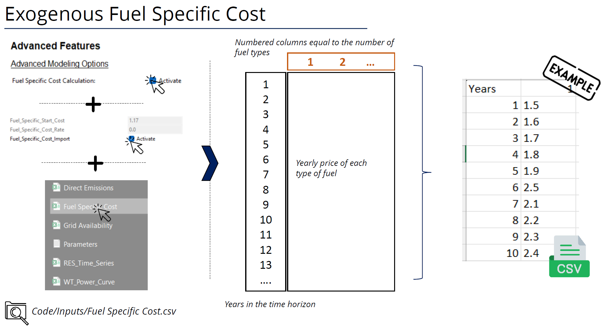
For the fuel-related parameters, the GUI provides tools for: - Setting the fuel types, lower heating value (LHV), specific CO2 emissions, and cost-related information. - If the Fuel Specific Cost Calculation feature is activated, the user must input fuel cost values into a CSV file located in the ‘Inputs’ folder. This feature takes into account the fluctuating costs of fuel over the project’s lifespan.
Lastly, for projects requiring an in-depth analysis of fuel cost over time, the GUI allows the importation of exogenous fuel cost data via a CSV file, which should contain yearly prices for each type of fuel considered over the project’s time horizon.
Running the Model
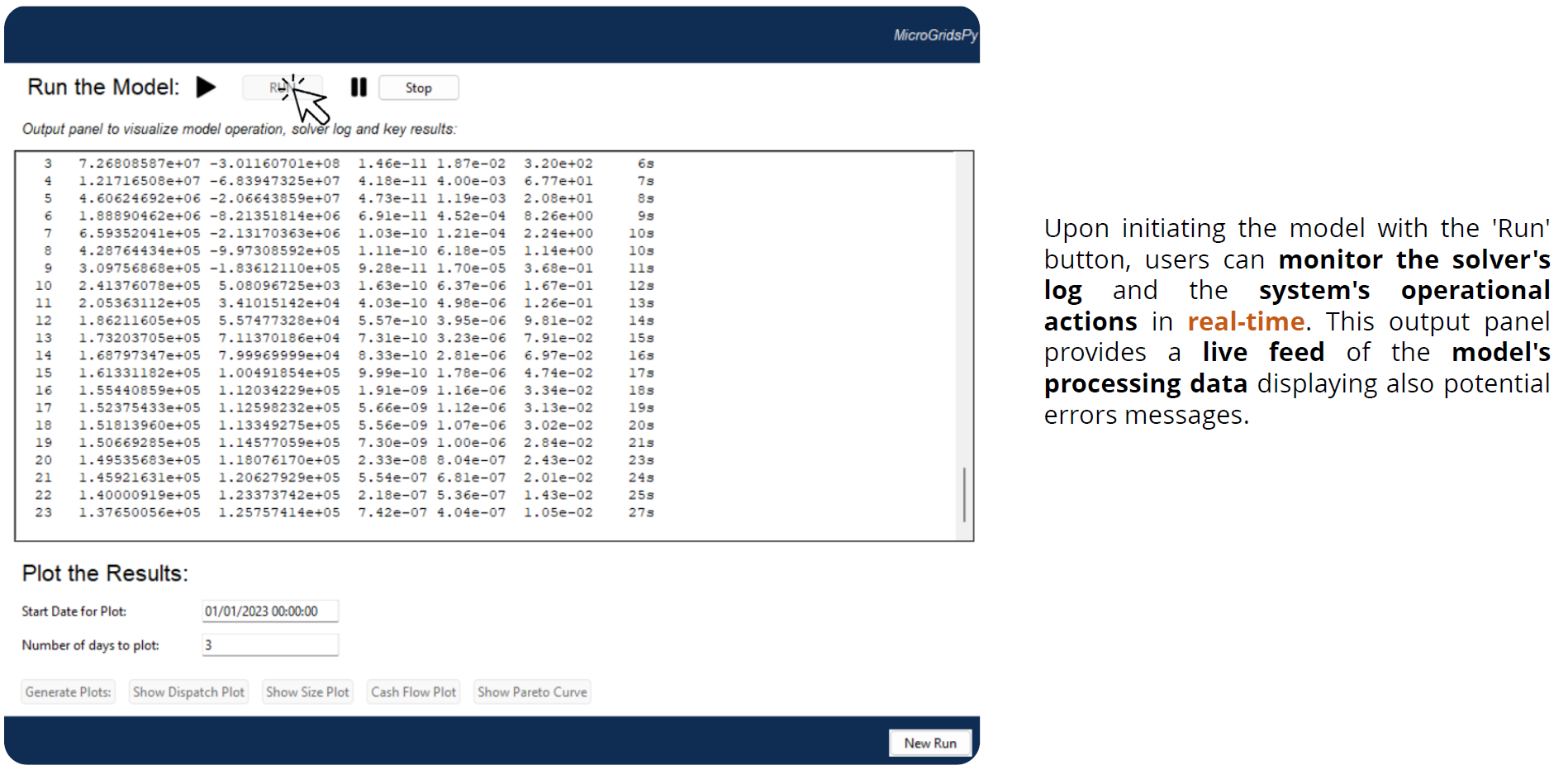
Pressing the Run but, the MicroGridsPy execution phase will start. Users can observe the solver’s log and system operations as the model runs. This process is fundamental for validating the simulation’s integrity and for immediate troubleshooting. A dedicated output panel displays the solver’s live log, offering real-time feedback on the model’s computations, including solver operations and key result indicators. Any errors or issues during the model run are also reported in this panel, allowing users to identify and address potential problems swiftly.
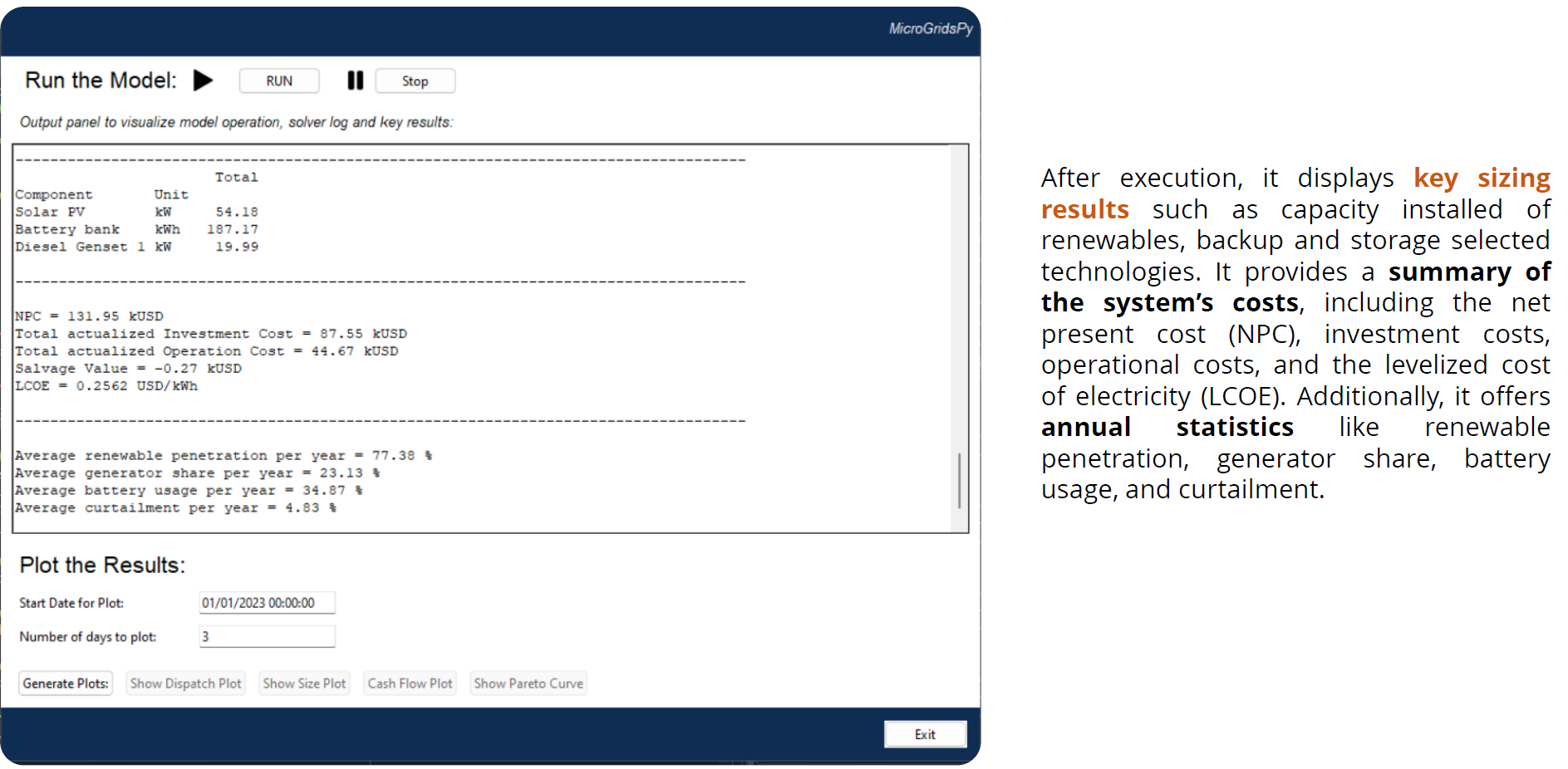
Once the model run is complete, the interface presents key sizing results and a comprehensive summary of system costs:
Users are provided with details such as installed capacities, lifecycle costs including net present cost (NPC), investment costs, operational costs, and the levelized cost of electricity (LCOE).
Annual statistics for renewable penetration, generator share, battery usage, and curtailment are also displayed, giving users a snapshot of the system’s yearly performance.
Obtaining the Results
The GUI provides functionality for plotting model outputs, enabling users to visualize the system’s performance over a selected timeframe.
By entering the start date and the number of days to plot, users can generate graphs for energy dispatch, system sizing, and financial analysis.
Graphs like the dispatch plot, size plot, cash flow plot, and Pareto curve offer a visual interpretation of the model’s operational dynamics and economic viability.
