Building and Running a Model
MicroGridsPy is a comprehensive energy optimization model designed for the strategic planning and operational management of mini-grid systems.
Here below is a general introduction to the different steps in building and running a model:
Time Series Data Input: Begin by providing specific data, over the lifetime of the project, about the available renewable resources and demand profiles. For sub-Sahara Africa it is also possible to estimate endogenously these time series data based on editable parameters and build-in load demand archetypes
Configuration and Optimization setup: Set the model’s general parameters, such as the number of periods (e.g., 8760 for hourly analysis) and the total duration of the project, specific features and modes such as MILP formulation, Multi-Objective optimization, Grid connection etc. as well as specific model’s optimization goals and constraints, such as aiming for a minimum renewable penetration or a certain level of battery independence.
Component Selection: Choose the technologies to include, like PV panels or wind turbines of a specific model, and define their capacities and operational characteristics.
Execution: Run the model to perform the optimization. MicroGridsPy processes the inputs through its algorithms to find the most cost-effective and efficient system setup.
Output Analysis: Review the outputs, which include the sizing of system components, financial analyses like NPC and LCOE, and dispatch plots.
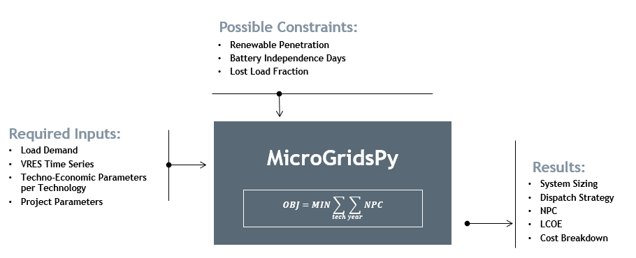
Simple scheme of the model
Energy System
The considered system comprises an electrical load supplied by renewable sources, an inverter, a battery bank and backup generators.
Renewable Generation Technologies
The system can incorporate an arbitrary number of renewable energy sources (RES), with the most common being:
Solar Power: Typically implemented using photovoltaic (PV) modules to convert sunlight into electricity.
Wind Power: Utilizing wind turbines to harness kinetic energy from wind currents.
MicroGridsPy allows for extensive modeling of these RES types, requiring users to input specific data for each technology’s parameters.
Storage System
The system employs a storage system to manage the energy balance:
Battery Bank: Often utilizing lead-acid or lithium-ion batteries, this storage system retains excess energy for use during periods of high demand or insufficient renewable generation.
In MicroGridsPy , the user can define and model a single battery bank system, inputting specific parameters to match the mini-grid’s requirements.
Backup Systems
To ensure reliability, the mini-grid can include an arbitrary number of backup systems (and related fuels), with the most common being:
Diesel Generator: Provides a conventional power generation solution during low production from renewable sources.
Biomass Micro-Turbine: Acts as a sustainable backup power source, converting biomass into electricity.
These backup systems are vital for continuous power supply and can be extensively modeled, similar to renewable technologies.

The interconnection of these components ensures that the electrical load is met with a combination of renewable energy sources, storage capacity, and backup systems, optimizing the use of sustainable energy and enhancing the reliability of the power supply. The configuration also allows for the management of energy flow to maximize efficiency and maintain balance between supply and demand.
Data Input Interface and Parameters
The graphical user interface (GUI) application provides a user-friendly way to define and input data for MicroGridsPy.
Run the app_main.py file located into the Code/User Interface folder using the prefered IDE (e.g. Spyder) to open the interface and interact with it.
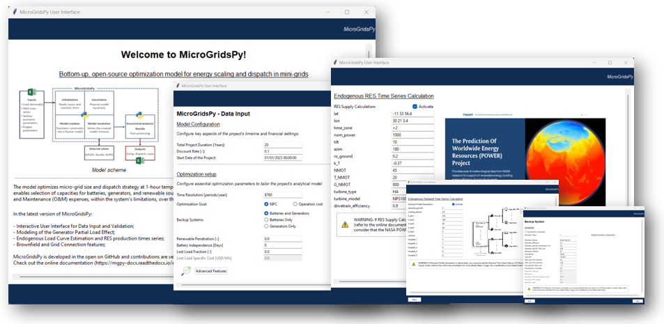
The application is organized into different pages, each tailored to a specific aspect of the model. Here’s a quick overview of the pages, their basic usage and the parameters included:
Initial Page: Initial page with the model presentation
Basic Parameter Initialization: Begin your data input journey by specifying fundamental parameters for your minigrid project. It serves as the central hub for configuring parameters and functionalities including duration, resolution, optimization goal,specific constraints and more.
Parameter name |
Unit |
Description |
|---|---|---|
Time Resolution |
Time unit (e.g. hours/year) |
Periods considered in one year (e.g. 8760 hours/year) |
Total Project Duration |
[years] |
Total duration of the project (or ‘time horizon’) |
Start Date |
‘DD/MM/YYYY hh:mm:ss’ |
Start date of the project |
Discount_Rate |
[%] (0-1) |
Real discount rate accounting also for inflation |
Optimization_Goal |
NPC / Operation cost |
It allows to switch between an NPC-oriented optimization and a NON-ACTUALIZED Operation |
Investment Cost Limit |
[USD] |
Upper limit to investment cost (considered only in case Optimization_Goal=’Operation cost’) |
Model_Components |
Batteries and Generators / Batteries only / Generators only |
It allows to switch between different configuration of backup system technologies (RES are always included) |
Renewable_Penetration |
[%] (0-1) |
Minimum renewable penetration (fraction of electricity produced by renewable sources) in the final technology mix |
Battery_Independence |
[days] |
Number of days of battery independence (working without backup choices) |
Lost_Load_Fraction |
[%] (0-1) |
Maximum admittable loss of load (between 0 and 1) |
Lost_Load_Specific_Cost |
[USD/Wh] |
Value of the unmet load |
Advanced Model Configuration: The GUI supports advanced modeling optimization features like mixed-integer linear programming (MILP) formulation, multi-objective optimization, and the ability to toggle different parameters: users can enable or disable specific parameters and access tooltips for additional guidance.
Note
Refer to (Advanced Features) for more detail information about all the additional model configuration parameters and their implementatiion within the model.
RES Time Series Data Simulation: Explore options for renewable energy time series estimation. Users can activate or deactivate RES calculation, which dynamically enables or disables related parameters. The layout offers a scrollable area for a comprehensive list of parameters, including latitude, longitude, time zone, and turbine information. Custom fonts and tooltips enhance the user experience, making it a user-friendly interface for setting up requried parameters.
Note
Refer to (Advanced Features) for all the additional model parameters and their implementatiion within the model. Refer to (Model Structure) for insights about the specific python module functioning
Archetypes Page: Simulate demand profiles and built-in archetypes referring to rural villages in Sub-Saharan Africa at different latitudes. These are composed of different types of end-users like households according to the wealth tier (i.e., from 1 to 5), hospitals with the same wealth scale and schools. The possibility for demand growth and specific cooling period are also integrated within this feature.
Note
Refer to (Advanced Features) for all the additional model parameters and their implementatiion within the model. Refer to (Model Structure) for insights about the specific python module functioning
Technologies Page: Configure the available renewable energy sources and their techno-economic properties. The page defines default parameters and their initial values for renewable energy sources (RES), manages user input for RES parameters with validation and updates, creates labels, entry fields, and tooltips for RES parameters.
Parameter name |
Unit |
Description |
|---|---|---|
RES_Sources |
[-] |
Number of Renewable Energy Sources (RES) types |
RES_Names |
(e.g. ‘PV panels’, ‘Wind turbines’) |
Renewable Energy Sources (RES) names |
RES_Nominal_Capacity |
Power (e.g. W) |
Single unit capacity of each type of Renewable Energy Source (RES) |
RES_Inverter_Efficiency |
[%] (0-1) |
Efficiency of the inverter connected to each Renewable Energy Source (RES) (put 1 in case of AC bus) |
RES_Specific_Investment_Cost |
[USD/W] |
Specific investment cost for each type of Renewable Energy Source (RES) |
RES_Specific_OM_Cost |
[%] (0-1) |
O&M cost for each type of Renewable Energy Source (RES) as a fraction of the specific investment cost |
RES_Lifetime |
[years] |
Lifetime of each Renewable Energy Source (RES) |
RES_unit_CO2_emission |
(e.g. kgCO2/kW) |
Emissions for each kW of capacity installed (indirect emissions) |
Battery Page: If needed, set up battery-related parameters. It provides robust input validation, tooltips for parameter descriptions, and conditional parameter handling, ensuring data accuracy and usability.
Parameter name |
Unit |
Description |
|---|---|---|
Battery_Specific_Investment_Cost |
[USD/Wh] |
Specific investment cost of the battery bank [USD/Wh] |
Battery_Specific_Electronic_Investment_Cost |
[USD/Wh] |
Specific investment cost of non-replaceable parts (electronics) of the battery bank |
Battery_Specific_OM_Cost |
[-] (0-1) |
O&M cost of the battery bank as a fraction of the specific investment cost |
Battery_Discharge_Battery_Efficiency |
[%] (0-1) |
Discharge efficiency of the battery bank |
Battery_Charge_Battery_Efficiency |
[%] (0-1) |
Charge efficiency of the battery bank |
Battery_Depth_of_Discharge |
[%] (0-1) |
Depth of discharge of the battery bank (maximum amount of discharge) |
Maximum_Battery_Discharge_Time |
[hours] |
Maximum time to discharge the battery bank |
Maximum_Battery_Charge_Time |
[hours] |
Maximum time to charge the battery bank |
Battery_Cycles |
[-] |
Maximum number of cycles before degradation of the battery |
Battery_Initial_SOC |
[%] (0-1) |
Battery initial state of charge |
BESS_unit_CO2_emission |
[kgCO2/kWh] |
Emissions for each kWh of capacity installed (indirect emissions) |
Generator Page: Define generator types and characteristics. Similarly to Technologies Page, the page defines default parameters and their initial values but the user can add new entries for different types of generators. It offers strong input validation, parameter description tooltips, and conditional parameter management.
Parameter name |
Unit |
Description |
|---|---|---|
Generator_Types |
[units] |
Number of different types of gensets |
Generator_Names |
(e.g. ‘Diesel Genset 1’) |
Generator names |
Generator_Efficiency |
[%] (0-1) |
Average generator efficiency of each generator type |
Generator_Specific_Investment_Cost |
[USD/W] |
Specific investment cost for each generator type |
Generator_Specific_OM_Cost |
[%] (0-1) |
O&M cost for each generator type as a fraction of specific investment cost [%] |
Generator_Lifetime |
[years] |
Lifetime of each generator type |
Fuel_Names |
(e.g. ‘Diesel’) |
Fuel names (to be specified for each generator, even if they use the same fuel) |
Fuel_Specific_Cost |
[USD/lt] |
Specific fuel cost for each generator type |
Fuel_LHV |
[Wh/lt] |
Fuel lower heating value (LHV) for each generator type |
GEN_unit_CO2_emission |
[kgCO2/kW] |
Emissions for each kW of capacity installed (indirect emissions) |
FUEL_unit_CO2_emission |
[kgCO2/lt] |
Emissions for each lt of fuel consumed (direct emissions) |
Grid Page: Specify grid connection details such the year starting from which the model should take account of the national grid connection and the possibility to simulate the grid availability by means of average quantities such as number of outages and duration in a year.
Plot Page: Visualize the color codes for data visualization by means of a dynamic color legend. These parameters are used for the aesthetic aspects of model outputs, assigning colors to different energy sources, storage options, and other model components for visual representation in plots and charts.
Parameter Name |
Default Value |
Description |
|---|---|---|
RES_Colors |
Coler hex code (e.g. ‘FF8800’) |
Color code for renewable energy sources in visualizations. |
Battery_Color |
Coler hex code (e.g. ‘4CC9F0’) |
Color code for battery storage in plots and graphs. |
Generator_Colors |
Coler hex code (e.g. ‘00509D’) |
Color codes for different types of generators in visualizations. |
Lost_Load_Color |
Coler hex code (e.g. ‘F21B3F’) |
Color code used for representing lost load in graphical outputs. |
Curtailment_Color |
Coler hex code (e.g. ‘FFD500’) |
Color code for curtailment in plots and diagrams. |
Energy_To_Grid_Color |
Coler hex code (e.g. ‘008000’) |
Color code for depicting energy supplied to the grid. |
Energy_From_Grid_Color |
Coler hex code (e.g. ‘800080’) |
Designates the color for visualizing energy drawn from the grid. |
Run Page: Finally, save your input data and initiate the optimization process. It includes the following functionalities: validation of integer inputs, updating and displaying output messages in a text widget, showing dispatch, size, and cash flow plots in separate windows, generating plots based on user inputs and running a model in a separate thread, displaying progress messages and results.
Parameter Name |
Default Value |
Description |
|---|---|---|
Start date for plot |
‘DD/MM/YYYY hh:mm:ss’ |
Starting day of the project time horizon to be displayed in the dispatch plot |
Number of days |
[-] |
Number of days to be displayed in the dispatch plot |
This intuitive interface streamlines the data input process, making it easier than ever to design and optimize minigrids for rural villages using MicroGridsPy.
Note
Please refer to the (Example Gallery) for a better understanding of the parameter use within the user interface.
Time Series Data
Demand
Introduction
At the core of the optimization energy modelling process lies the load curve demand. This section aims to explain what load curve demand is, how it is used within MicroGridsPy, and how it can be operated or estimated with external software tools like RAMP or within the model itself using the advanced feature of demand estimation integrated into MicroGridsPy.
What is the load curve demand?
Load Curve Demand represents the time-dependent electricity consumption of a given area or system. It is typically measured in Watts (or kilowatts, megawatts, etc.) and captures how electricity demand varies over different periods, usually in hourly or sub-hourly intervals. MicroGridsPy uses the load curve demand to optimize resource allocation, distributing resources efficiently over the years. The software can predict when investment steps should be taken to expand the system’s capacity for increasing demand.
MicroGridsPy uses the load curve demand to optimize resource allocation, distributing resources efficiently over the years. It balances generation and storage resources to minimize costs while meeting the electricity demand throughout the day. The software can predict when investment steps should be taken to expand the system’s capacity for increasing demand.
Load curve demand estimation methods:
Using software tools such as RAMP, a bottom-up stochastic model for generating high-resolution multi-energy profiles.
Using the advanced features integrated into MicroGridsPy, which allows the use of built-in archetypes for rural villages in Sub-Saharan Africa at different latitudes.

Demand.csv
The input file, located in the “Time Series” folder within the “Inputs” folder, must have as many numbered columns (excluding the rows labels) as the total years of the project and as many rows (excluding the columns headers) as the periods in which one year is divided (e.g. 1-hour time resolution leads to 8760 rows).
Warning
The number of columns in the csv file must coincide with the value set for the ‘Years’ parameter. The same for the number of rows that must coincide with the value set for ‘Periods’ in the model configuration.csv file! If not properly set and matched, it may arise a ‘Key Error’.
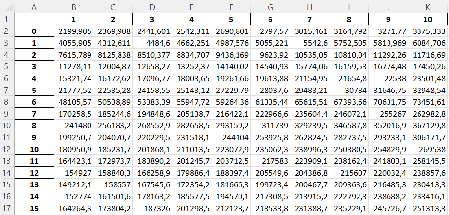
Example of demand csv file structure
RES Production
Introduction
Electricity needed to meet the demand can be generated using various energy sources. MicroGridsPy considers renewable sources, such as solar and wind, and backup diesel generators as the choices for generating electricity. This section aims to explain what renewable energy production is, how it is used within MicroGridsPy, how it can be estimated with external available web tools like Renewables.ninja and PVGIS or within the model itself using the advanced feature of renewable energy production estimation integrated into MicroGridsPy.
What is the Renewable energy production?
Renewable energy production represents the estimated electricity production for each unitary generation technology at a specific time and location. It is typically measured in Watts (or kilowatts, megawatts, etc.) and illustrates how electricity production varies over time and by source, usually in hourly or sub-hourly intervals.
MicroGridsPy uses this data to size and operate mini-grid components like renewable energy sources (e.g., solar panels, wind turbines), energy storage systems (e.g., batteries), and backup generators to ensure necessary electricity for a specific area or community.
Renewable Energy Production estimation methods:
Using web tools such as Renewables.ninja, which provides data and tools for assessing energy generation profiles, including solar and wind energy production estimated for 1 year with 1-hour time resolution.
Using the advanced features integrated into MicroGridsPy for estimating generation based on VRES parameters, project location, and the specific year. Data for solar, wind, and temperature conditions are obtained from the NASA POWER platform through an API integrated into the MGPy software, creating a Typical Meteorological Year (TMY) dataset for energy generation calculations.
RES_Time_Series.csv
The input file within the “Inputs” folder, must have as many numbered columns (excluding the rows labels) as the total years of the project and as many rows (excluding the columns headers) as the periods in which one year is divided (e.g. 1-hour time resolution leads to 8760 rows).
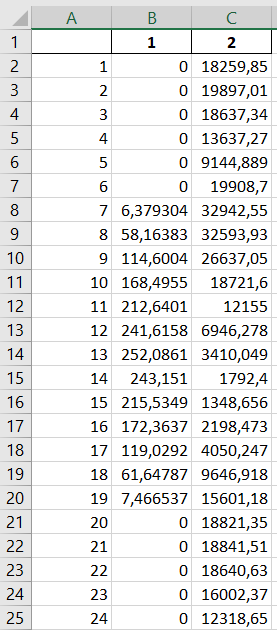
Example of the RES Time Series csv file structure